Artificial intelligence (AI) is revolutionizing the world, impacting everything from healthcare to entertainment. At the heart of AI is machine learning, a subset that enables computers to learn from data. But how do these machines actually learn? One of the most fundamental techniques used in machine learning is gradient descent. This optimization algorithm is essential for training AI models, helping them to become more accurate and efficient. Let’s dive into the world of gradient descent and understand how it optimizes AI learning.

What is Gradient Descent?

Gradient descent is an optimization algorithm used to minimize the cost function in machine learning and deep learning. The cost function, also known as the loss function, measures how well the model predicts the target values. In simpler terms, gradient descent helps to adjust the model parameters (weights and biases) to reduce the difference between the predicted and actual values.

Imagine you are hiking down a mountain with your eyes closed, and you want to reach the lowest point (the global minimum). You take small steps in the direction that reduces your elevation the most. This is analogous to gradient descent, where the algorithm takes small steps in the direction that reduces the cost function the most.

How Does Gradient Descent Work?

Gradient descent works by iteratively adjusting the model parameters to find the minimum of the cost function. Here’s a step-by-step explanation:

1. Initialize Parameters: Start by initializing the model parameters (weights and biases) with random values.
2. Calculate the Cost: Compute the cost function using the current parameters.
3. Compute the Gradient: Calculate the gradient of the cost function with respect to each parameter. The gradient is a vector of partial derivatives, indicating the direction and rate of the steepest increase in the cost function.
4. Update Parameters: Adjust the parameters in the opposite direction of the gradient. The size of the step is determined by the learning rate, a hyperparameter that controls how big the steps are.
5. Repeat: Repeat steps 2-4 until the cost function converges to a minimum value or reaches a predefined number of iterations.

Types of Gradient Descent

There are several variants of gradient descent, each with its own advantages and drawbacks:

Batch Gradient Descent

Batch gradient descent computes the gradient using the entire training dataset. While it provides a precise gradient estimate, it can be computationally expensive and slow for large datasets. However, it tends to converge smoothly to the minimum.

Stochastic Gradient Descent (SGD)

Stochastic gradient descent updates the model parameters using a single training example at each iteration. This makes it much faster than batch gradient descent, but the gradient estimates are noisier, leading to more fluctuations in the cost function. Despite this, SGD can help escape local minima and find the global minimum.

Mini-Batch Gradient Descent

Mini-batch gradient descent is a compromise between batch gradient descent and SGD. It splits the training dataset into small batches and updates the parameters for each batch. This approach provides a balance between the efficiency of SGD and the smooth convergence of batch gradient descent.

Learning Rate: The Critical Hyperparameter

The learning rate is a crucial hyperparameter in gradient descent. It determines the size of the steps taken towards the minimum of the cost function. If the learning rate is too high, the algorithm may overshoot the minimum and fail to converge. Conversely, if the learning rate is too low, the algorithm will take tiny steps and require more iterations to converge, making the training process slow.

Choosing an appropriate learning rate is essential for the efficiency and performance of the model. Techniques such as learning rate schedules and adaptive learning rates (e.g., Adam, RMSprop) can help optimize the learning rate during training.

The Mathematics Behind Gradient Descent

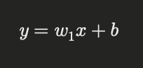
To truly appreciate gradient descent, it’s helpful to understand the mathematical principles behind it. Let’s consider a simple linear regression model with a single feature:

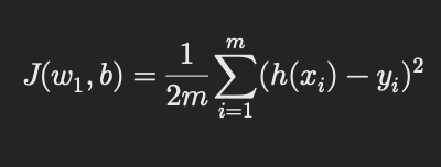
Here, ( y ) is the predicted value, ( w_1 ) is the weight, ( x ) is the input feature, and ( b ) is the bias. The cost function (mean squared error) for this model is:

where ( h(x_i) = w_1 x_i + b ), and ( m ) is the number of training examples.

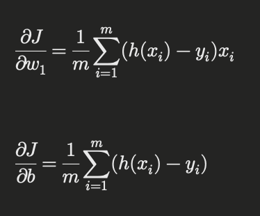
The goal of gradient descent is to minimize ( J(w_1, b) ). To do this, we need to compute the partial derivatives of ( J ) with respect to ( w_1 ) and ( b ):

Using these gradients, we update the parameters:

Here, ( \alpha ) is the learning rate.

Challenges and Solutions in Gradient Descent

While gradient descent is a powerful optimization algorithm, it comes with its own set of challenges:

Local Minima and Saddle Points

One of the main challenges in gradient descent is the presence of local minima and saddle points. Local minima are points where the cost function is lower than neighboring points but higher than the global minimum. Saddle points are points where the gradient is zero but are not minima or maxima.

Solution: Using stochastic gradient descent or adding noise to the gradient can help the algorithm escape local minima and saddle points. Additionally, advanced optimization algorithms like Adam and RMSprop can handle these issues more effectively.

Choosing the Right Learning Rate

As mentioned earlier, choosing an appropriate learning rate is crucial. An improper learning rate can lead to slow convergence or divergence.

Solution: Experimenting with different learning rates and using techniques like learning rate schedules or adaptive learning rates can help find the optimal learning rate.

Feature Scaling

Features with different scales can cause gradient descent to converge slowly or fail to converge.

Solution: Normalizing or standardizing the features ensures that they have a similar scale, improving the efficiency of gradient descent.

Advanced Gradient Descent Techniques

Several advanced techniques have been developed to improve the performance and efficiency of gradient descent:

Momentum

Momentum helps accelerate gradient descent by adding a fraction of the previous update to the current update. This technique helps the algorithm converge faster and reduce oscillations.

Here, ( v_t ) is the velocity, ( \beta ) is the momentum factor, and ( \theta ) represents the model parameters.

Nesterov Accelerated Gradient (NAG)

NAG is an improvement over momentum, where the gradient is calculated at the estimated next position of the parameters. This results in more accurate updates and faster convergence.

AdaGrad

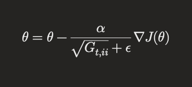
AdaGrad adapts the learning rate for each parameter based on the historical gradients. This makes it well-suited for sparse data and helps in dealing with varying feature scales.

where ( G_t ) is a diagonal matrix of the sum of the squares of the historical gradients, and ( \epsilon ) is a small constant to avoid division by zero.

RMSprop

RMSprop addresses the diminishing learning rate problem in AdaGrad by using a moving average of the squared gradients.

Adam

Adam (Adaptive Moment Estimation) combines the benefits of momentum and RMSprop. It computes adaptive learning rates for each parameter and has been widely adopted due to its efficiency and performance.

Practical Applications of Gradient Descent

Gradient descent is a cornerstone of many machine learning and deep learning applications:

Image Recognition

Gradient descent is used to train convolutional neural networks (CNNs) for image recognition tasks. These models can identify objects, faces, and scenes with high accuracy, powering applications like self-driving cars, medical image analysis, and facial recognition systems.

Natural Language Processing (NLP)

In NLP, gradient descent is used to train models for tasks such as sentiment analysis, machine translation, and text classification. Models like recurrent neural networks (RNNs) and transformers rely on gradient descent to learn patterns and relationships within textual data, enabling applications like chatbots, automated translation, and content recommendation.

Speech Recognition

Gradient descent plays a crucial role in training models for speech recognition. These models can transcribe spoken words into text, making them essential for virtual assistants like Siri, Alexa, and Google Assistant, as well as for automated customer service systems.

Recommendation Systems

E-commerce platforms, streaming services, and social media networks use recommendation systems to personalize content for users. Gradient descent optimizes these models to provide accurate and relevant recommendations based on user behavior and preferences.

Financial Modeling

In finance, gradient descent helps train models for predicting stock prices, assessing credit risk, and detecting fraud. These applications require highly accurate predictions, and gradient descent ensures that the models learn from historical data effectively.

Tips for Implementing Gradient Descent

Implementing gradient descent effectively requires careful consideration of various factors. Here are some tips to ensure successful optimization:

Initialize Parameters Wisely

Proper initialization of model parameters can significantly impact the convergence speed and final performance. Techniques like Xavier initialization and He initialization are commonly used to set initial values that are neither too large nor too small.

Choose an Appropriate Learning Rate

As discussed earlier, the learning rate is critical. Use techniques like grid search, random search, or Bayesian optimization to find the optimal learning rate. Additionally, employ learning rate schedules or adaptive learning rate algorithms to adjust the rate dynamically during training.

Monitor the Training Process

Track the training progress by monitoring the cost function and evaluation metrics. Visualize the learning curves to identify potential issues like overfitting, underfitting, or divergence. Early stopping can be used to halt training if the model stops improving on the validation set.

Regularize the Model

Regularization techniques like L1, L2, and dropout can prevent overfitting by penalizing large parameter values or randomly dropping units during training. This ensures that the model generalizes well to unseen data.

Use Gradient Clipping

Gradient clipping prevents the gradients from becoming too large, which can cause the model parameters to diverge. This is especially useful in training deep networks or recurrent neural networks where gradient explosion is a common issue.

Future Directions in Gradient Descent

As machine learning and AI continue to evolve, so do the optimization techniques. Here are some future directions and advancements in gradient descent:

Advanced Optimization Algorithms

Researchers are continually developing new optimization algorithms that build on gradient descent. These algorithms aim to improve convergence speed, stability, and performance. Techniques like Lookahead optimizer, LARS (Layer-wise Adaptive Rate Scaling), and NovoGrad are gaining attention for their potential to enhance training efficiency.

Quantum Gradient Descent

Quantum computing is an emerging field that promises to revolutionize optimization in machine learning. Quantum gradient descent leverages quantum algorithms to solve optimization problems faster and more accurately than classical methods. While still in its infancy, this approach holds great potential for the future of AI.

Automated Machine Learning (AutoML)

AutoML aims to automate the process of model selection, hyperparameter tuning, and optimization. Gradient descent plays a pivotal role in AutoML frameworks, enabling the automatic optimization of models without human intervention. As AutoML advances, it will make AI accessible to a broader audience, democratizing machine learning.

Federated Learning

Federated learning allows multiple devices to collaboratively train a model without sharing raw data. Gradient descent is used to update the global model by aggregating the gradients computed on individual devices. This approach enhances privacy and security while leveraging distributed data for training.

Conclusion

Gradient descent is the backbone of many machine learning and deep learning algorithms. Its ability to optimize model parameters and minimize the cost function makes it indispensable for training accurate and efficient AI models. Understanding the different types of gradient descent, their challenges, and advanced techniques can help you implement this powerful algorithm effectively.

As AI continues to advance, so will the optimization techniques that drive its progress. By staying informed about the latest developments and best practices in gradient descent, you can harness the full potential of this essential algorithm to build smarter, more capable AI systems.

Disclaimer: The information provided in this blog is for educational purposes only. While we strive for accuracy, please report any inaccuracies so we can correct them promptly.